BOFlow: Exploration-Aware Bayesian Optimisation in Workflow Space
About:
- Full title: BOFlow: Exploration-Aware Bayesian Optimisation in Workflow Space for Agent Evolution.
- Accepted at ACL Rolling Review (ARR) — the commitment venue is not finalised yet, and the paper is not public. Please treat the numbers below as a pre-publication write-up.
- Authors: Shashwat Gupta (me), Anson Bastos, Xuchao Zhang, Ritabrata Maiti, Chetan Bansal.
- Presented at the day-long AICE Conference at UIUC, 10 September 2026.
- Headline result: ~10% average accuracy gain over state-of-the-art automated workflow-design baselines across eight benchmarks (77.7 → 89.2 average).
- arXiv / camera-ready PDF: not yet public.
- Code: not yet public.
- This blog is my own write-up of the motivation, the design choices we made, and what the numbers actually say. It is written to be readable without the paper in front of you.
The one-paragraph version
Agentic workflows — the structured composition of LLM calls, tool invocations and control logic that sits behind any serious agent — are still mostly hand-built. The obvious fix is to search for them automatically, and prior work does exactly that: ADAS generates and evaluates candidate pipelines, AFlow represents workflows as code graphs and runs Monte Carlo Tree Search over them. These methods work, but they lean on the LLM itself as the explorer, and LLMs are not built for structured discrete optimisation. The search keeps rediscovering variations of whatever worked first. We call this what it is: structural mode collapse.
BOFlow takes the other road. We treat workflow discovery as a black-box optimisation problem, embed each code-represented workflow into a continuous feature space, fit a Gaussian Process surrogate over performance in that space, and select the next candidate using both Expected Improvement and an explicit KNN-based novelty term. The LLM stays in the loop — but as a domain-aware generator and selector, not as the optimiser. Across eight reasoning, QA and code-generation benchmarks this lifts the average from 77.7 (AFlow) to 89.2, while exploring 3–4× more of the workflow space and sitting on the cost–performance Pareto frontier.
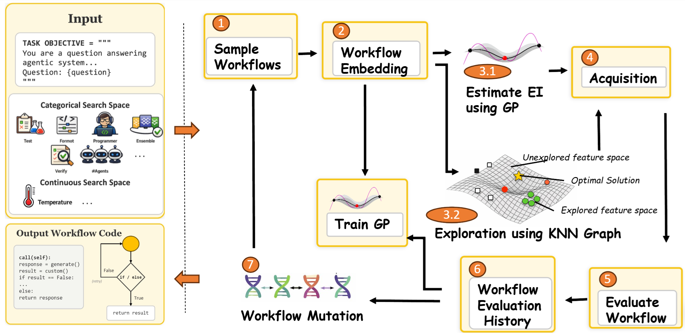
Figure 1: The BOFlow loop. Workflows are sampled and embedded (1–2); a GP estimates Expected Improvement while a KNN graph scores novelty (3.1–3.2); an LLM policy picks the next candidate (4); it is executed (5), written into evaluation memory (6), and that memory conditions the next round of LLM-guided mutation (7).
Motivation: why does workflow search collapse?
The search space is genuinely nasty
A workflow is a directed acyclic graph of operators — a reasoning step, an ensemble, a verifier, a programmer step, a retry loop. That gives you a space that is combinatorial, non-smooth, and expensive to evaluate: every single candidate costs you multiple LLM executions, and what comes back is a sparse, noisy scalar. You cannot brute-force it, you cannot differentiate through it, and you get very few samples.
Using an LLM as the optimiser makes it worse
When the proposal distribution is the LLM's prior, the optimiser inherits the LLM's biases. Ask a model to "improve this workflow" thirty times and it will keep reaching for the same handful of patterns it has seen most often in training. Combine that with a greedy selection rule and you get premature convergence: the search parks itself in one region and stops asking whether a structurally different workflow would do better. This matters most exactly where you would want the search — complex tasks, where several genuinely distinct workflow structures can reach comparable scores and only sustained exploration finds the good ones.
So the thing we actually needed was a global model of the search landscape — something that knows where it has already been, and can quantify how uncertain it is about where it has not. That is a textbook description of Bayesian optimisation. The reason nobody had done it here is representational: BO wants continuous inputs, and workflows are discrete programs.
Formulating it
Let $\mathcal{G}$ be the space of valid agent workflows, where each $g \in \mathcal{G}$ is a DAG of LLM operators and control logic that compiles to an executable program. Each workflow has a score
$f(g) \in [0,1]$
obtained by running it on a held-out evaluation set. Evaluating $f$ is expensive and stochastic. Under a fixed budget of $T$ evaluations we want
$g^{*} = \arg\max_{g \in \mathcal{G}} f(g)$.
The move that unlocks everything else is a mapping
$\phi : \mathcal{G} \rightarrow \mathbb{R}^{d}$
which embeds a workflow into a $d$-dimensional space capturing its structural and semantic properties. This does two jobs at once: it lets us put a continuous surrogate model on top, and it gives us a notion of similarity between workflows — which is what we later use to measure whether the search is actually exploring.
The method, piece by piece
Bootstrapping the surrogate
A GP with no observations is useless, so we start with a warm-up phase of $T_0$ evaluations of a template workflow $g_0$ and minor variants of it (generated by prompting the LLM), producing an initial dataset $\mathcal{D}_t = \{(g_i, x_i, f(g_i))\}_{i=1}^{t}$ with $x_i = \phi(g_i)$. This is the cheapest possible way to give the surrogate enough signal to estimate both a mean and an uncertainty — and without the uncertainty, the acquisition step is meaningless.
A candidate pool with memory
Each round we generate a pool $\mathcal{P} = \{g_1, \dots, g_K\}$ by LLM-guided mutation of the current best workflow $g^{*}_{\text{curr}}$. The difference from prior work is the memory buffer $\mathcal{M}$: it stores what happened in previous rounds — structural patterns that worked, mutations that failed — and gets injected into the mutation prompt. The LLM is therefore conditioned on the trajectory of the search, not just on its current best point.
The embedding $\phi$
$\phi$ is deliberately lightweight: a composition of static program analyses over the workflow code. It captures structural signals (number of operators, workflow depth), execution-level properties (number of LLM calls, whether verification or testing steps are present) and control-flow patterns.
Crucially we do not treat these dimensions as a fixed, hand-weighted schema. The GP is retrained on the accumulated $\mathcal{D}_t$ each round, so the kernel implicitly learns which dimensions predict performance; useful directions get reinforced through the acquisition step and redundant ones get down-weighted. The representation adapts to the task rather than being specified for it.
Gaussian Process surrogate and Expected Improvement
We place a GP prior over $f$ in the embedding space, $f(x) \sim \mathcal{GP}(m(x), k(x,x'))$, giving the usual posterior
$\mu_t(x) = k(x,X)^{\top}(K + \sigma_n^2 I)^{-1} y$, $\sigma_t^2(x) = k(x,x) - k(x,X)^{\top}(K + \sigma_n^2 I)^{-1} k(x,X)$
and then compute Expected Improvement over the current best $f^{+} = \max_{i \le t} f(g_i)$:
$\mathrm{EI}(x) = \left(\mu(x) - f^{+}\right)\Phi(Z) + \sigma(x)\,\varphi(Z)$, $Z = \dfrac{\mu(x) - f^{+}}{\sigma(x)}$
EI already trades off exploitation (high predicted score) against exploration (high uncertainty). But in a high-dimensional structured space, EI on its own still drifts towards regions the surrogate already knows well — because that is where its estimates are confident enough to look attractive. That drift is the mechanism of structural collapse.
KNN exploration regularisation — the part that actually fixes collapse
So we add an explicit novelty term. For a candidate embedding $x$, let $N_k(x)$ be its $k$ nearest neighbours among the already-evaluated workflows:
$\mathrm{Div}(x) = \dfrac{1}{k}\displaystyle\sum_{i \in N_k(x)} \lVert x - x_i \rVert_2$
normalised to $[0,1]$ across the candidate set. The intuition is simple and, I think, the conceptual core of the paper: distance in the workflow embedding space is a proxy for "structurally different hypothesis". A candidate far from everything we have tried is not just a perturbation of the incumbent — it is a different idea about how to solve the task. Rewarding that distance is how the search climbs out of a local optimum.
Acquisition: an LLM policy rather than a fixed formula
Classical BO combines acquisition signals with a fixed functional form. We found that the right balance between improvement and novelty varies both across tasks and across stages of a single run — early on you want coverage, later you want refinement. So the primary policy $\psi$ hands the decision to the LLM:
$g_t = \psi(\mathcal{T}, \mathcal{M})$
where $\mathcal{T} = \{(g_j, x_j, \mathrm{EI}(x_j), \mathrm{Div}(x_j))\}_{j=1}^{K}$ is the scored candidate set and $\mathcal{M}$ is the evaluation memory. The LLM sees the numbers and the history, and picks. This is the one place where "LLM as optimiser" is actually the right tool — it is a small, well-posed, context-rich choice, not an open-ended search.
To make the contribution of each signal measurable, we also implement a deterministic fallback policy:
$g_t = \arg\max_{g \in \mathcal{P}} \; \lambda_1 \mathrm{EI}(x_j) + \lambda_2 \mathrm{Div}(x_j)$
which is what the $\lambda$ ablations below run on.
Reflect–repair
A selected workflow is first executed on a small set of validation examples. If it errors, the execution feedback goes back to the LLM, which reflects on the failure and revises the workflow; this can repeat for a few iterations and yields extra candidates for the next round. It is a cheap trick with an outsized effect — it converts execution failures, which are otherwise just a zero in the dataset, into a usable learning signal.
Putting it together
1. Warm-up: evaluate $T_0$ variants of the template workflow $g_0$; build $\mathcal{D}_0$.
2. for $t = 1 \dots T$ do
3. Fit the GP surrogate on $\mathcal{D}_t$.
4. Generate pool $\mathcal{P}$ by LLM-guided mutation of $g^{*}_{\text{curr}}$, conditioned on memory $\mathcal{M}$.
5. for each candidate $g_j \in \mathcal{P}$: embed $x_j = \phi(g_j)$; compute $\mathrm{EI}(x_j)$ and $\mathrm{Div}(x_j)$; add to $\mathcal{T}$.
6. Select $g_t = \psi(\mathcal{T}, \mathcal{M})$.
7. Reflect–repair, then evaluate $f(g_t)$.
8. Update $\mathcal{D}_{t+1}$, $\mathcal{M}$, and the running best.
9. return the best workflow observed.
Read as a loop over rounds, this is agent evolution: the workflow the agent runs is progressively rewritten by the optimiser, and the improvement is driven by measured performance rather than by a human's guess about what should help.
Experiments
We asked three questions. RQ1: how does BOFlow compare to automated workflow-design baselines? RQ2: how much does each component matter? RQ3: how token-efficient is it?
Datasets. Eight benchmarks spanning reasoning, QA and code generation: GSM8K, MATH, HumanEval, MBPP, HotpotQA, DROP, BBH and MMLU-Pro. Following prior work on automated workflow optimisation we split each dataset into validation and test at a 1:4 ratio. Full test sets are used for GSM8K, HumanEval and MBPP; HotpotQA and DROP are subsampled to 1,000 instances each; MATH uses the standard 617-problem protocol over representative categories; BBH and MMLU-Pro use a 500-sample held-out test set with a 50–200 sample optimisation set.
Baselines. Manually designed prompting strategies (direct IO, Chain-of-Thought, self-consistent CoT, MedPrompt, Multi-Persona Debate, Self-Refine) and automated workflow optimisers (ADAS, AFlow, ShinkaEvolve, GEPA).
Setup. To keep the comparison honest we adopt the same experimental setup as AFlow: all workflows are executed with GPT-4o-mini as the underlying model, under a fixed optimisation budget. Every workflow is evaluated three times (seeds 40, 41, 42); we report mean and standard deviation. Metrics are the standard ones per task — solve rate for GSM8K and MATH, pass@1 for HumanEval and MBPP, F1 for HotpotQA and DROP, exact match for BBH and MMLU-Pro.
Results
| Method | HotpotQA | DROP | HumanEval | MBPP | GSM8K | MATH | BBH | MMLU-Pro | Avg |
|---|---|---|---|---|---|---|---|---|---|
| IO (GPT-4o-mini) | 71.9 | 73.0 | 87.8 | 73.3 | 88.5 | 41.0 | 45.6 | 39.6 | 65.1 |
| CoT | 71.5 | 79.3 | 87.7 | 74.8 | 89.2 | 39.9 | 47.2 | 40.0 | 66.2 |
| CoT SC (5-shot) | 71.6 | 80.5 | 88.6 | 72.1 | 93.6 | 42.6 | 46.0 | 43.0 | 67.2 |
| MedPrompt | 70.9 | 73.1 | 88.6 | 71.6 | 91.2 | 44.7 | 46.4 | 32.8 | 64.9 |
| MultiPersona | 67.2 | 81.0 | 90.1 | 72.1 | 93.2 | 43.8 | 68.4 | 36.6 | 69.0 |
| Self-Refine | 66.3 | 70.1 | 93.9 | 69.5 | 69.4 | 46.8 | 70.4 | 61.6 | 68.5 |
| ADAS | 78.1 | 81.5 | 87.9 | 75.6 | 92.2 | 33.6 | 38.4 | 36.6 | 65.5 |
| AFlow | 77.8 | 87.2 | 94.3 | 89.5 | 95.8 | 54.6 | 54.0 | 68.6 | 77.7 |
| ShinkaEvolve | 73.2 | 83.3 | 87.0 | 86.5 | 94.9 | 52.7 | 57.2 | 65.2 | 79.6 |
| GEPA | 73.7 | 80.5 | 88.1 | 84.8 | 93.3 | 52.7 | 71.6 | 39.2 | 73.0 |
| BOFlow (ours) | 82.9 | 91.9 | 95.9 | 96.5 | 96.7 | 75.1 | 86.8 | 88.0 | 89.2 |
BOFlow is best on all eight benchmarks. The improvements are statistically significant ($t$-test, $p < 0.05$) everywhere except HumanEval and GSM8K, which are close to saturated for this model class — and I would rather say that plainly than claim a win where the headroom does not exist.
The interesting pattern is where the gains concentrate. On MATH (54.6 → 75.1), BBH (54.0 → 86.8) and MMLU-Pro (68.6 → 88.0) — the tasks that need multi-stage reasoning and where several distinct workflow structures are plausible — the margin is 20–30 points. On tasks with one obvious workflow shape, everything converges to roughly the same place. That is exactly the signature you would predict if the bottleneck in prior methods were exploration rather than proposal quality.
We also compare against MaAS (AgentSupernet), a cost-aware state-of-the-art method, on the four shared benchmarks: BOFlow leads on all of them (GSM8K 96.5 vs 92.3, MATH 70.2 vs 51.82, HumanEval 95.1 vs 92.85, MBPP 95.7 vs 82.17). Worth being precise about the claim though: MaAS optimises execution cost explicitly and BOFlow does not, so the two address complementary objectives and could be composed rather than treated as rivals.
Ablations: which parts carry the weight?
| Configuration | MATH | GSM8K | HotpotQA |
|---|---|---|---|
| BOFlow (LLM acquisition) | 75.1 | 96.7 | 82.9 |
| argmax acquisition, $\lambda_1 = \lambda_2 = 1$ | 68.5 | 93.5 | 80.7 |
| No diversity ($\lambda_2 = 0$) | 68.1 | 92.6 | 76.7 |
| High diversity ($\lambda_2 = 2$) | 68.7 | 93.5 | 80.4 |
| No Bayesian optimisation | 67.5 | 93.5 | 70.1 |
| No reflect–repair | 68.7 | 93.3 | 75.0 |
Four things fall out of this table:
- The GP is the load-bearing component. Removing Bayesian optimisation causes the largest drop across the board — HotpotQA falls from 82.9 to 70.1. Without a surrogate there is no global model of the landscape, and the search is back to heuristics.
- LLM acquisition beats argmax. Delegating selection to the LLM over the scored candidate set is worth roughly 6.6 points on MATH over the best fixed-$\lambda$ rule. The fixed rule cannot re-balance exploration against exploitation as the run progresses; the policy can.
- Diversity matters, but it is not a dial you crank. Setting $\lambda_2 = 0$ hurts most on HotpotQA (76.7), the most open-ended, multi-hop task — which is precisely where alternative structures exist to be found. But doubling it to $\lambda_2 = 2$ buys nothing: 68.7 on MATH, and HotpotQA actually slips to 80.4. Novelty is a corrective term, not an objective.
- Reflect–repair earns its place. Removing it costs ~6.4 points on MATH and ~7.9 on HotpotQA, confirming that recovering signal from failed executions is not a nice-to-have.
How many dimensions does $\phi$ need?
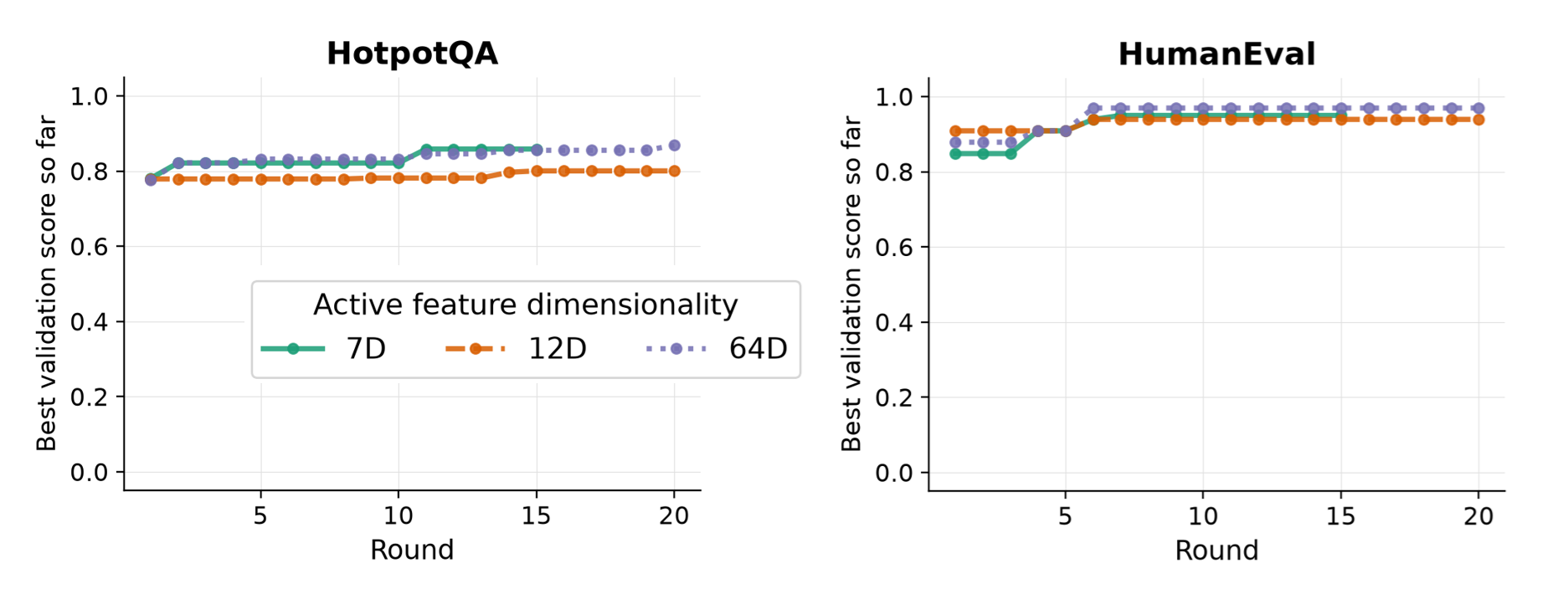
Figure 2: Best validation score vs. optimisation round for 7D, 12D and 64D active feature dimensionality.
The honest answer is: less than you would expect, and the optimum is dataset-dependent. HotpotQA converges fastest at 7 dimensions (around round 12); HumanEval converges fastest at 64 dimensions (around round 7). But the final performance differences are marginal — BOFlow is robust to this choice, which was a relief, because a method that needs its embedding dimension tuned per task would be much less useful in practice.
Does it actually explore more? (the mode-collapse analysis)
This is the experiment I care about most, because it tests the paper's central claim directly rather than through the proxy of accuracy. We embed workflows from both AFlow and BOFlow using the same $\phi$ — AFlow's are embedded post hoc, so its own optimisation procedure is untouched — reduce each to a 7-dimensional structural descriptor, and project to 2D with t-SNE for a shared visualisation space.
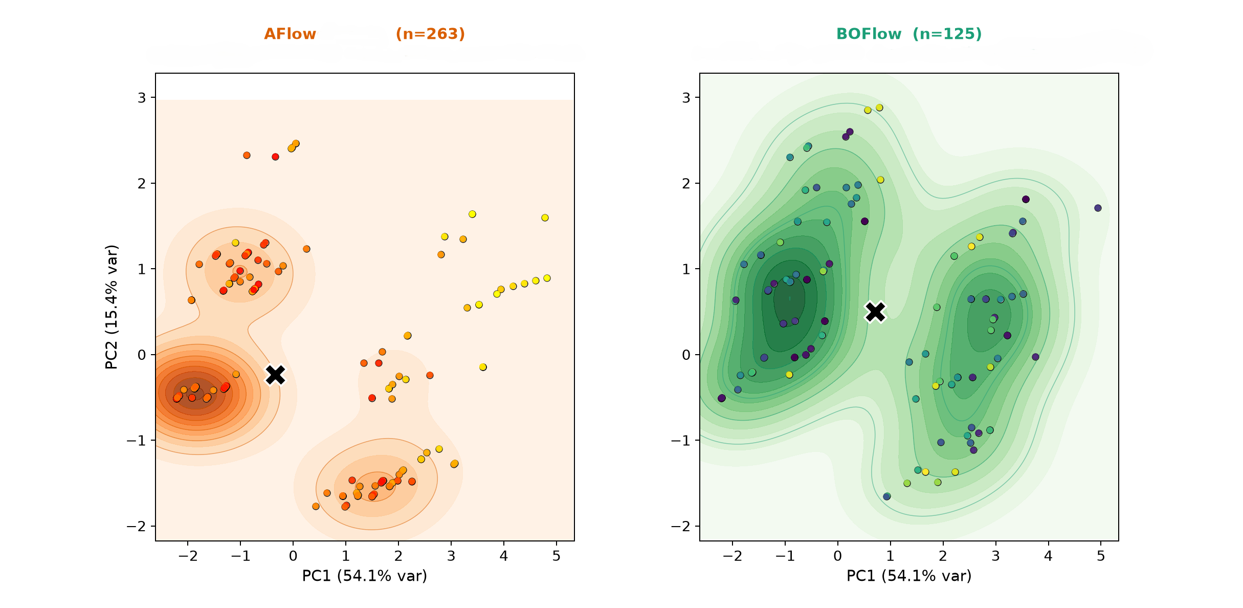
Figure 3: Each point is a workflow, coloured by iteration order. AFlow (left) concentrates in a narrow region — structural collapse. BOFlow (right) spreads across multiple distinct modes.
AFlow's workflows pile into one dominant cluster: the search keeps sampling minor variations of a small number of templates. BOFlow's are distributed across several regions. Measured as the volume of the convex hull of the sampled points, BOFlow covers 3–4× more of the space — while evaluating fewer workflows (131 vs 263).
| Method | n | Mean pairwise GED | Std |
|---|---|---|---|
| AFlow | 263 | 6.15 | 4.44 |
| BOFlow | 131 | 37.79 | 59.08 |
The t-SNE picture could be an artefact of the projection, so we also measure structural diversity directly: mean pairwise graph-edit distance between the workflows' abstract syntax trees. BOFlow's is 37.79 vs AFlow's 6.15 — more than a six-fold increase, on half the evaluation budget. The much larger standard deviation (59.08 vs 4.44) is itself informative: it says BOFlow produces both incremental refinements and structurally distinct solution families, which is the behaviour you want from a search that is meant to generate hypotheses rather than polish one.
Cost
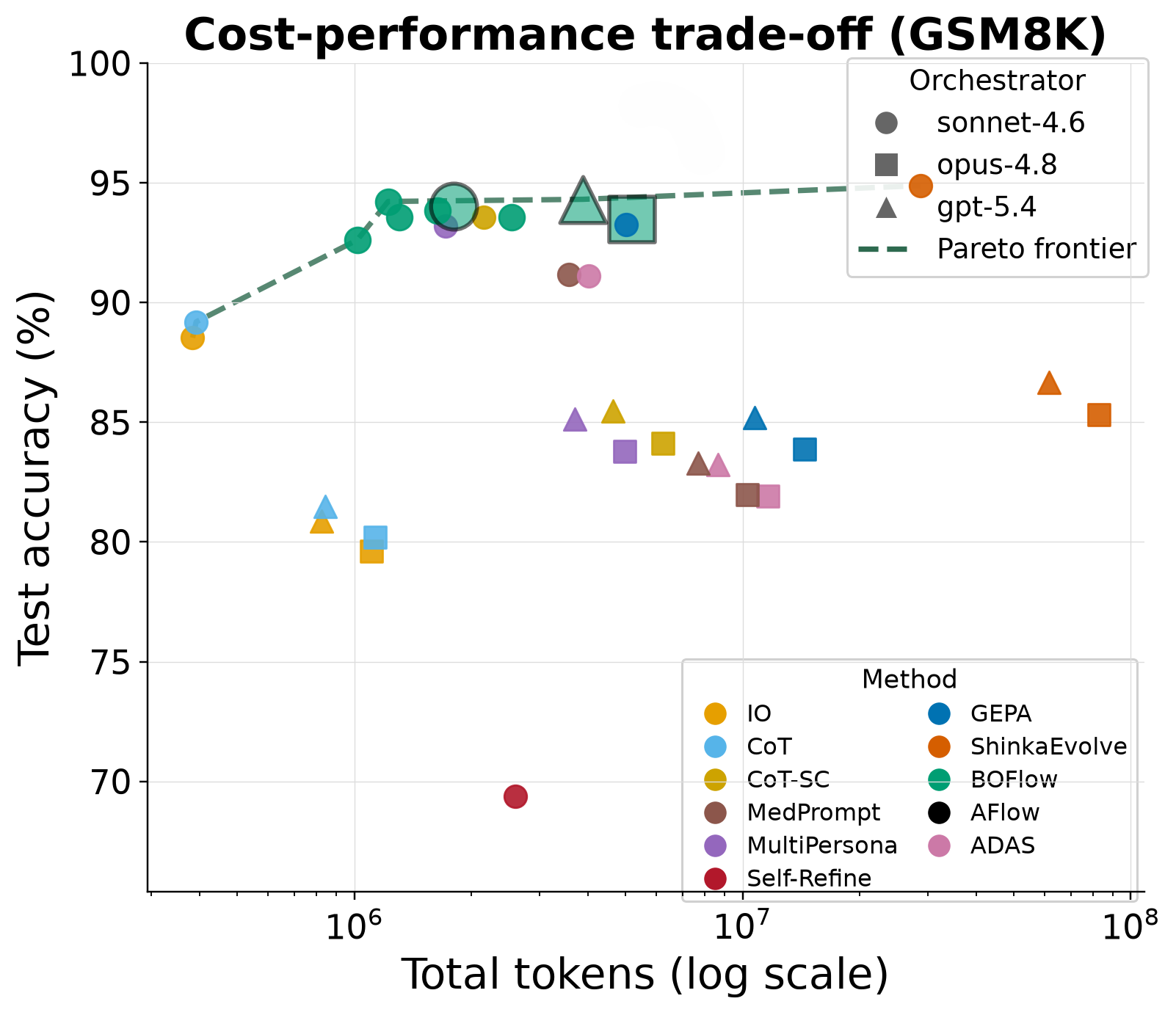
Figure 4: Cost–performance trade-off on GSM8K. BOFlow lies on the Pareto frontier.
A method that gets better answers by burning ten times the tokens is not obviously progress, so we plotted test accuracy against total tokens on GSM8K. BOFlow sits on the Pareto frontier, attaining higher pass@1 at both low- and medium-cost regimes and avoiding the dominated configurations that several baselines occupy.
There is a nice reason for this, and it is not an accident: diversity-aware search does not only find better workflows, it finds cheaper ones. If you only ever mutate the incumbent, complexity ratchets upwards — every improvement adds a step. If you are rewarded for jumping to structurally distinct regions, simple-but-effective configurations stay reachable.
Case study: what evolution actually looks like
We traced a single 30-round run on GSM8K. Workflows there are built from operators such as
Custom (a basic reasoning step), ScEnsemble (an ensemble over
multiple LLM outputs) and Programmer (a computation-oriented step).
The winning trajectory runs from a simple seed at R1 (0.875) to the best workflow at R19 (0.972). Along the way the workflow acquires ensembling, then parallel reasoning branches, and finally — between R8 and R19 — the initial ensemble is replaced by a computation-driven step, which is what produces the best configuration in the run. Note that the last move is a substitution, not an addition: the search removed a component it had earlier added. Greedy incremental mutation does not do that.
The dashed alternatives in the same run are a useful corrective against over-reading the result — R3 and R16 collapsed to 0.0, R26 landed at 0.769. Only a small fraction of explored workflows lie on the improvement path. The search space is high-variance and unforgiving; the value of the surrogate is that it makes the failures cheap and informative rather than merely wasted.
What I would take away from this
- Give the LLM the job it is good at. LLMs are excellent domain-aware generators and good at small, context-rich choices. They are not structured discrete optimisers. Splitting those roles — LLM proposes and selects, GP models the landscape — is most of the win.
- You cannot fix collapse you cannot measure. The embedding $\phi$ is the enabling trick, but its second job — giving us a distance between workflows — is what let us define $\mathrm{Div}$, diagnose AFlow's collapse quantitatively, and report GED. A representation you can measure in is worth more than a representation that is merely expressive.
- Exploration is a regulariser, not an objective. $\lambda_2 = 0$ hurts and $\lambda_2 = 2$ does not help. The useful framing is that novelty exists to stop EI from over-trusting the region it already understands.
- Failures are data. Reflect–repair was the cheapest component to build and one of the most valuable, because in a sparse-feedback setting a crashed workflow otherwise teaches you almost nothing.
Limitations and where this goes next
- All main-table results use GPT-4o-mini as the execution model, matching AFlow's protocol for comparability. Generalisation across orchestrator models is something we probe but do not exhaustively characterise.
- The embedding $\phi$ is a set of static program analyses. It is deliberately cheap, and the GP learns which dimensions matter — but a learned or semantic embedding of workflow code is an obvious next step.
- BOFlow optimises for task performance, not execution cost. The Pareto result is a by-product of diversity, not the result of a cost-aware objective; combining BOFlow's search with an explicitly cost-aware method such as MaAS is the natural composition.
- GP surrogates scale awkwardly with the number of observations. Under the evaluation budgets that workflow search actually has (order 10–100 evaluations) this is a non-issue, but it bounds how far the approach stretches.
References
[1] Hu et al. (2024). Automated Design of Agentic Systems (ADAS).
[2] Zhang et al. (2025). AFlow: Automating Agentic Workflow Generation. ICLR 2025.
[3] Zhuge et al. (2024). GPTSwarm: Language Agents as Optimizable Graphs. ICML 2024.
[4] Liu et al. (2023). DyLAN: Dynamic LLM-Agent Network.
[5] Lange et al. (2025). ShinkaEvolve.
[6] Agrawal et al. (2025). GEPA: Reflective Prompt Evolution.
[7] Zhang et al. (2025). MaAS / AgentSupernet: Multi-agent Architecture Search.
[8] Snoek et al. (2012). Practical Bayesian Optimization of Machine Learning Algorithms. NeurIPS 2012.
[9] Jones et al. (1998). Efficient Global Optimization of Expensive Black-Box Functions. Journal of Global Optimization.
[10] Srinivas et al. (2012). Information-Theoretic Regret Bounds for Gaussian Process Optimization.
[11] Wei et al. (2022). Chain-of-Thought Prompting Elicits Reasoning in Large Language Models. NeurIPS 2022.
[12] Wang et al. (2023). Self-Consistency Improves Chain of Thought Reasoning. ICLR 2023.
[13] Madaan et al. (2023). Self-Refine: Iterative Refinement with Self-Feedback. NeurIPS 2023.
[14] Shinn et al. (2023). Reflexion: Language Agents with Verbal Reinforcement Learning. NeurIPS 2023.
[15] van der Maaten & Hinton (2008). Visualizing Data using t-SNE. JMLR.