A queuing theory primer, and where these rules came from

Both policies in this post are older than the hardware they now run on, and knowing where they came from tells you what they assume.

The vocabulary. A queue is described in Kendall's notation as A/S/c: arrival process, service distribution, number of servers. M/M/1 is Poisson arrivals, exponential service, one server. M/G/1 relaxes the service distribution to anything with a finite mean and variance, which is the case that matters here, because LLM service times are emphatically not exponential. Write $\lambda$ for arrival rate, $\mu$ for service rate, and $\rho = \lambda/\mu$ for utilisation. The system is stable only when $\rho < 1$.

Little's law (Little, 1961) is the one result you can never escape: $\mathbb{E}[L] = \lambda \mathbb{E}[T]$, the average number in the system equals arrival rate times average time in the system. It needs almost no assumptions, which is why it is the bridge between "holding cost" as an economist writes it and "latency" as an SRE measures it. Minimise one and you have minimised the other.

The Pollaczek-Khinchine formula gives M/G/1 waiting time as $\mathbb{E}[W] = \lambda \mathbb{E}[S^2] / (2(1-\rho))$. Two things fall out of it immediately, and both govern everything below. First, the $1/(1-\rho)$ term: delay does not grow linearly with load, it blows up near saturation. Second, it depends on $\mathbb{E}[S^2]$, the second moment: variance in service time hurts you directly. A workload with the same mean but a fatter tail is strictly worse, and LLM output lengths have a fat tail. That single fact is most of why scheduling matters here at all.

WSPT comes from Wayne Smith in 1956, in a paper about single-stage production scheduling in a factory. The problem was which order to run jobs on a machine, and the answer, now called Smith's rule, was ratio order by $w_j/p_j$. It is a deterministic, offline, single-machine result, and section 3 gives the proof.

The c-mu rule comes from Cox and Smith in 1961, in the monograph Queues, and is the stochastic online counterpart: with random arrivals and random service you cannot order a fixed list, so instead you fix a priority among classes, and the optimal priority is by $c_k \mu_k$. Klimov, and later the achievable-region and polymatroid literature, generalised it and explained why a greedy index is optimal rather than merely observing that it is.

Deficit Round Robin, which section 10 pairs with them, comes from somewhere else entirely: Shreedhar and Varghese, SIGCOMM 1995, solving fair packet scheduling in network routers, where the problem was giving each flow a guaranteed share of a link without per-packet sorting. It is a fairness mechanism, not an efficiency one, which is precisely why it composes well with an index rule instead of competing with it.

So a modern LLM router is running a 1956 factory heuristic inside a 1995 router-fairness algorithm, over a 1961 queueing model. The reason that works is that none of these results are about factories, packets, or tokens. They are about a scarce server and a queue of things that want it.

The problem

A router-scheduler for LLM serving answers two questions on two timescales. On the slow timescale, minutes to hours, it decides how much capacity to place where: how many GPUs of which SKU, in which region, for which model. On the fast timescale, milliseconds, it decides which request to serve next and on which endpoint. The slow loop is a forecasting and provisioning problem and is naturally an integer program. The fast loop is a queuing problem, and that is this post.

Set it up as a multiclass queue. Requests arrive of class $k$, each class carrying a holding cost (or weight) $w_k$ encoding how much you care about latency for that class, and a service time distribution with mean $1/\mu_k$. Interactive chat is expensive to delay; an overnight batch summarisation is not. Writing $C_j$ for the completion time of request $j$, the objective almost every practical system is really optimising is

$$\min \sum_j w_j C_j$$

which in steady state becomes the long-run average holding cost $\sum_k w_k \mathbb{E}[L_k]$, with $L_k$ the number of class $k$ requests in the system. Little's law, $\mathbb{E}[L_k] = \lambda_k \mathbb{E}[T_k]$, says minimising holding cost and minimising weighted mean sojourn time are the same problem.

WSPT, and why it is optimal

Weighted Shortest Processing Time schedules in decreasing order of the ratio $w_j / p_j$, where $p_j$ is the processing time. For the deterministic single-machine problem $1 \,||\, \sum w_j C_j$ with all jobs available at time zero, WSPT is exactly optimal. This is Smith's rule, from 1956, and the proof is a two-line interchange argument worth seeing, because it tells you precisely what the rule trades off.

Notice what the argument does not need: no arrival process, no distributional assumption, no convexity. It needs only that $w/p$ is known. That is the entire catch, and section 6 is about the fact that in LLM serving it is not.

The c-mu rule

The c-mu rule is the stochastic counterpart. At each decision point, serve a request from the non-empty class maximising $c_k \mu_k$, holding cost times service rate. Cox and Smith showed this minimises long-run average holding cost for a multiclass M/G/1 queue. Since $\mu_k = 1/\mathbb{E}[p_k]$, the index $c_k \mu_k = w_k / \mathbb{E}[p_k]$ is WSPT applied to class means rather than individual jobs. Same idea, two granularities, and the difference matters more than it looks.

The deeper reason c-mu is optimal is a conservation law. For a work-conserving M/G/1 queue the workload in the system is the same under every non-idling policy: scheduling cannot create or destroy work, only decide who waits. Formally the achievable region of $(\mathbb{E}[L_1], \ldots, \mathbb{E}[L_K])$ is a polymatroid, and minimising a linear objective over a polymatroid is solved by a greedy index rule. c-mu is that greedy rule. This also names the price: you are not making the system faster, you are choosing who absorbs the delay. Figure 2 is that sentence as a bar chart.

For non-preemptive priorities, with classes ordered by priority and $\rho_k = \lambda_k / \mu_k$,

$$\mathbb{E}[W_k] = \frac{\sum_{j} \lambda_j \mathbb{E}[p_j^2] / 2} {\left(1 - \sum_{j < k}\rho_j\right)\left(1 - \sum_{j \le k}\rho_j\right)}$$

Both denominators shrink as load rises, so delay for low-priority classes grows roughly like $1/(1-\rho)^2$. Priority decisions matter far more at high utilisation than at low, which is why the curves in figure 1 fan out to the right instead of running parallel.

Where c-mu stops being optimal, which is most of the interesting cases: with convex holding costs it generalises to the generalised c-mu rule, optimal only asymptotically in heavy traffic; with abandonment the index becomes $c\mu/\theta$; with hard deadlines it is not optimal at all; and with multiple heterogeneous servers it stops being an index problem, because you must also decide where, not only who. Every one of those is live in LLM serving.

The other policies worth knowing

• FCFS: the work-conserving reference. Fair, trivial to implement, no starvation, and it discards every bit of information you have about weights and sizes.
• SRPT: preemptively serve the shortest remaining processing time. Optimal for mean flow time, famously strong, but it needs exact remaining sizes and starves long jobs.
• Processor sharing and round robin: what continuous batching gives you by default. Fair, needs no size information, and mean response time is insensitive to the service distribution beyond its mean, which is a real robustness property.
• JSQ and power of two choices: for the routing half. Sampling two endpoints and taking the shorter queue buys a doubly exponential improvement in maximum queue length over random, at a fraction of JSQ's coordination cost. Figure 5.

Why LLM serving breaks the assumptions

WSPT needs $p_j$. In LLM inference the service time is dominated by output token count, which is not known until the request finishes. You can predict it, and people do, but then WSPT is only as good as the predictor. That is measurable, and figure 4 measures it.

Four more things break:

• Prefill and decode differ. Prefill is compute bound and roughly quadratic in prompt length; decode is memory bandwidth bound and linear in output length. A single scalar $p_j$ is already a simplification.
• Continuous batching makes $\mu$ endogenous. Service rate depends on what else is in the batch, so $\mu_k$ is not a constant of the class but a function of the scheduling decision. The clean c-mu argument assumes it is not.
• The KV cache is a knapsack constraint. Admission is limited by memory as well as compute, adding a packing problem that queuing theory does not see.
• Demand is strongly non-stationary. Enterprise traffic is diurnal and regional. A policy tuned for the mean is tuned for a load level that is rarely the current one.

Those five facts are the argument for the architecture: a slow loop that forecasts demand (ARIMA is a reasonable choice for strongly seasonal, mostly linear traffic, and it is cheap to refit) and solves an integer program for placement, feeding a fast loop that applies an index policy to whatever capacity the slow loop provisioned. The slow loop absorbs non-stationarity and heterogeneity, which index rules handle badly. The fast loop handles instantaneous priority, which integer programs handle far too slowly.

The experiment

Three classes chosen to resemble real serving traffic: interactive ($w = 8$, mean service 0.30), standard ($w = 2$, mean 1.00), batch ($w = 0.5$, mean 4.00), arriving 50 / 35 / 15. Service times are lognormal rather than exponential, because output-length distributions have a long right tail and that tail is exactly what stresses a scheduler. 120,000 requests per configuration, first 20,000 discarded as warmup.

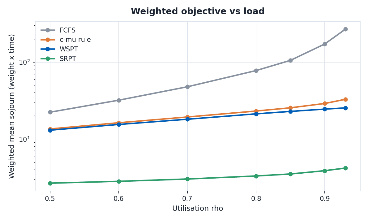
Figure 1. The weighted objective against load. At $\rho = 0.85$ the c-mu rule cuts it from 105.2 to 25.4, a 76% reduction, and job-level WSPT reaches 22.8, a 78% reduction. The gap widens with load, as the $1/(1-\rho)^2$ term predicts. SRPT sits far below everything else, but see section 8.

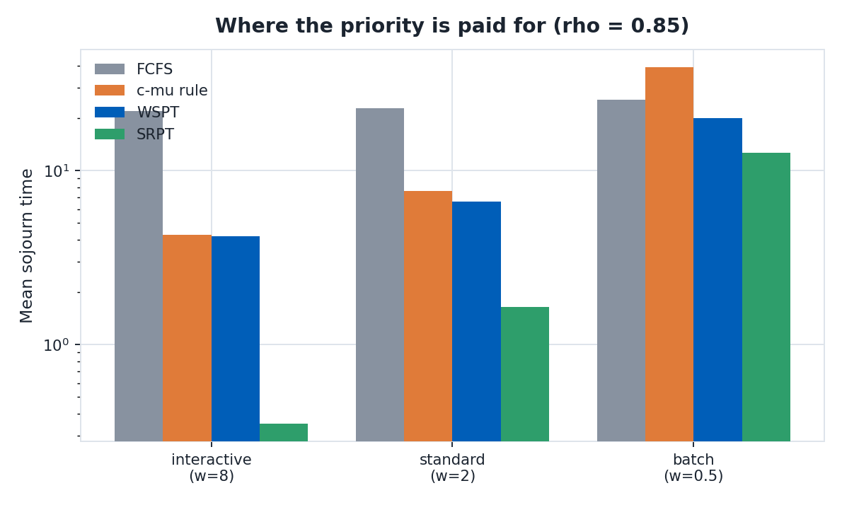
Figure 2. The conservation law made visible. FCFS gives every class roughly the same sojourn time (21.9 interactive, 25.5 batch). The c-mu rule takes interactive down to 4.28 and pays for it by pushing batch to 39.3, worse than batch got under FCFS. Nothing was created. Work was moved. This is the most important plot on the page, because it says a scheduling win is always a redistribution, and you had better agree with the direction of the transfer.

Note also that WSPT holds interactive at 4.17, essentially matching c-mu, while leaving batch at 20.0 rather than 39.3. Job-level sizing lets a short batch job overtake a long one; class-level c-mu cannot see the difference. That is the practical argument for building a size predictor.

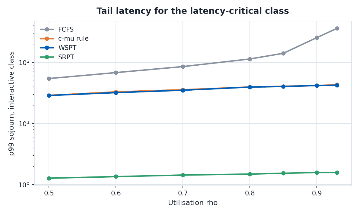
Figure 3. The p99 of the latency-critical class, which is what an SLA is actually written against. At $\rho = 0.85$ FCFS puts interactive p99 at 140.3 while c-mu holds it at 40.5. Means understate the benefit: priority helps the tail more than the average, because the tail is dominated by the times a short request queued behind a long one, which is exactly the event an index rule prevents.

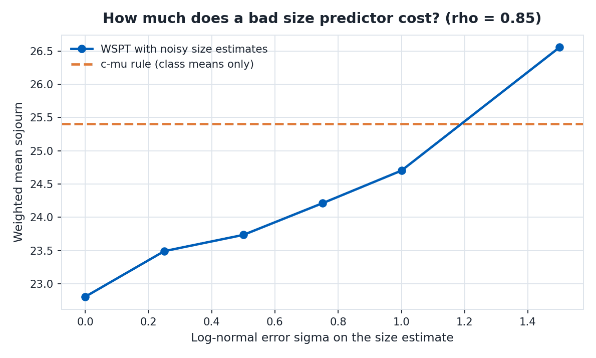
Figure 4. The plot that decides whether to build a predictor at all. WSPT is given size estimates corrupted by lognormal multiplicative noise of scale $\sigma$. With perfect estimates it scores 22.8. At $\sigma = 1.0$, a genuinely bad predictor, it degrades only to 24.7, and even at $\sigma = 1.5$ it is 26.6, still better than the c-mu baseline. WSPT degrades gracefully. The reason is in the interchange argument: the cost of a mis-ordered pair is $w_a p_b - w_b p_a$, which goes to zero as the pair becomes closer in ratio. Errors that reorder nearly equivalent jobs cost nearly nothing; only errors large enough to invert genuinely different jobs are expensive. You do not need a good predictor, you need one that is right about the big gaps.

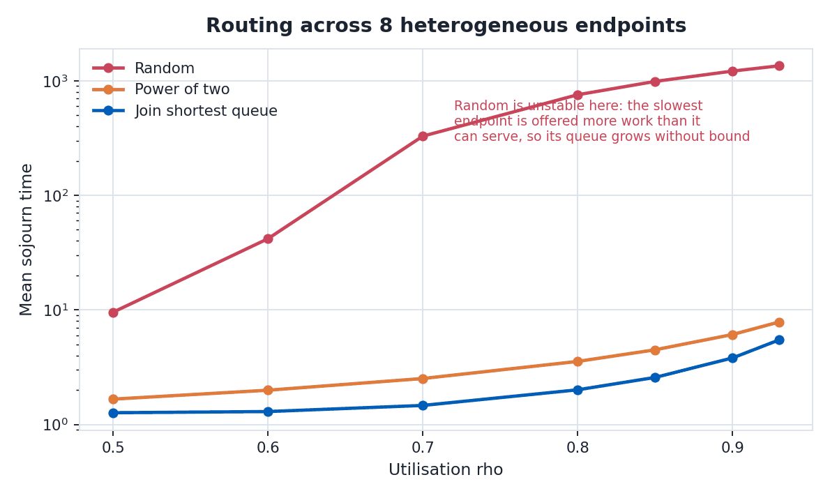
Figure 5. The routing half, across eight endpoints with speeds from 0.6 to 1.4. Random dispatch is not merely worse, it is unstable: it offers every endpoint an equal share, which is more work than the slowest can serve, so that queue grows without bound and the plotted value is an artefact of a finite run rather than a steady state. Join-shortest-queue gives 2.57 and sampling just two endpoints gives 4.48, most of the benefit for a fraction of the coordination. Heterogeneity is why a production router cannot be stateless.

Reading the results honestly

SRPT wins this benchmark and you should still be suspicious of it. It looks dominant in figures 1 and 2 partly because of how I set the problem up: here the high-weight class is also the short class, so shortest-first and highest-weight-first agree. Decouple them, make the expensive class the long one, and SRPT stops looking clever. It also assumes exact remaining sizes, precisely what LLM serving does not give you, and it starves long jobs in a way that surfaces as a support ticket rather than in this plot.

The c-mu rule is the one I would deploy first. It needs only per-class mean service rates, estimable from a day of logs; it has no per-request predictor to train, serve, or monitor for drift; and figure 2 shows it captures most of the available gain. WSPT is the upgrade you buy afterwards, and figure 4 says that upgrade is robust enough to be worth buying.

What this does not show. A single-server multiclass simulation with an exogenous service distribution. It does not model continuous batching, KV-cache pressure, prefill and decode asymmetry, or the slow provisioning loop. Each would change the numbers. It is a study of the policy question in isolation, which is all it claims to be.

What the theory says about the production design

• Because of the conservation law, no fast-loop policy reduces total work. If you need headroom rather than a different distribution of pain, the only lever is the slow loop: provision more, or provision it in the right place. That is what makes the integer program load-bearing and the index rule cheap.
• Because delay scales like $1/(1-\rho)$ and priority effects like $1/(1-\rho)^2$, a small reduction in effective utilisation buys a disproportionate latency improvement. Forecasting well enough to keep $\rho$ off the knee is worth more than any cleverness at $\rho$ close to one.
• Because index rules assume a single homogeneous server, and real fleets are heterogeneous and regional, placement genuinely has to be solved as an optimisation problem rather than approximated by a rule of thumb.

Which is the honest summary of the design: forecast demand, solve for placement on the slow loop, let a cheap index policy run the fast loop. The 6% recorded in production is a systems result from that whole pipeline. The figures here are a separate, reproducible argument for why the fast loop is shaped the way it is.

Where this shows up in practice: NVIDIA Dynamo

None of this is only theory. NVIDIA Dynamo, the open-source distributed inference serving framework, ships Smith's rule as a first-class router option. Its documentation names it directly: --router-queue-policy wspt, described as "WSPT (weighted shortest processing time, Smith's rule)", ordering requests by

$$\frac{1 + \texttt{priority\_jump}}{\texttt{isl\_tokens}}$$

which is exactly $w/p$ with the input sequence length standing in for the processing time and a priority jump standing in for the weight. The alternative, fcfs, orders by adjusted arrival time, priority_jump - arrival_offset. Dynamo's own framing is that WSPT optimises average time to first token while FCFS optimises tail TTFT. Section 11 tests that claim.

Above the ordering policy, Dynamo arbitrates between named policy classes with a work-conserving Deficit Round Robin variant. Its documented example classes are premium and regular: exactly the dual-load split most production deployments end up with. Each class carries a quantum "measured in uncached tokens" and a deficit of earned but unspent credit; on each ring round a class receives a quantum and dispatches if its head-of-line request is now affordable, against a scheduling cost of scheduling_cost = max(1, uncached_tokens). DRR decides which class goes next; FCFS or WSPT decides who inside that class goes next.

That is a clean separation of the two questions, and it is worth naming why it is the right one. The c-mu rule answers "who next" optimally but says nothing about guaranteeing a class a share of capacity, because a strict index rule will happily starve a class forever. DRR supplies exactly what c-mu lacks: a guaranteed floor, tunable per class. The pairing is DRR for isolation, WSPT for efficiency within an isolated slice.

The dual-load experiment: premium and regular

I reimplemented that structure to measure both knobs separately: two classes, premium at 30% of arrivals with a priority jump of 3, regular at 70% with none; lognormal input sequence lengths (means 700 and 1200 tokens) served at 3000 tokens per second; DRR arbitration with the documented max(1, uncached_tokens) cost; and FCFS or WSPT inside each class. Code in router_dual_class_sim.py, raw output in router_dual_class_results.json. This is a clean-room reimplementation of the public Dynamo design, not a model of any internal system.

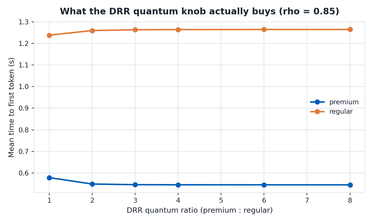
Figure 6. The DRR quantum ratio, swept from 1:1 to 8:1. Premium mean TTFT moves from 0.579s to 0.545s while regular moves from 1.238s to 1.264s. The striking thing is how fast it saturates: essentially all the available separation is bought by 2:1, and 8:1 is indistinguishable from 3:1. Once a class's quantum comfortably exceeds its head-of-line cost it is already dispatching whenever it has work, and further credit buys nothing. If you are tuning this knob past about 3:1 and expecting more, the lever you actually want is admission control or capacity, not quantum.

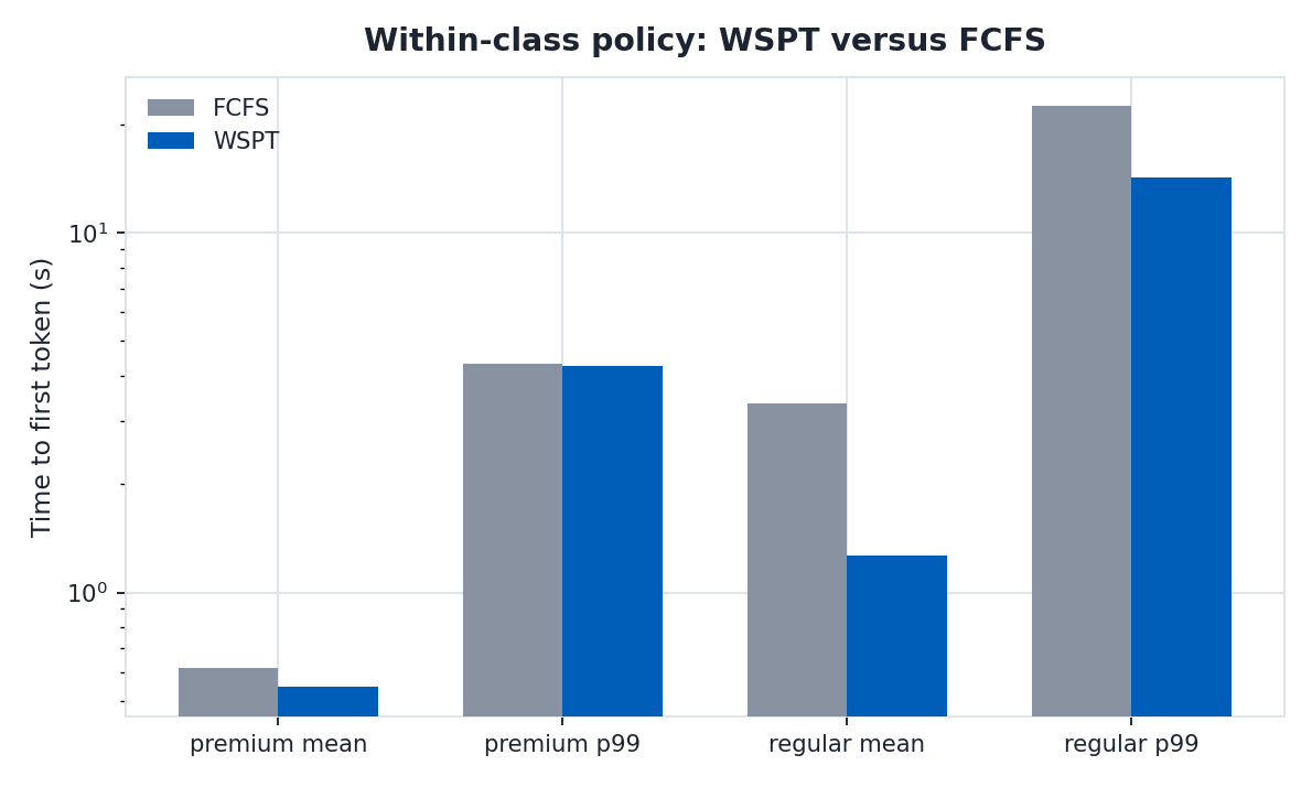
Figure 7. Within-class policy at a 4:1 quantum. WSPT beats FCFS on premium mean (0.546s against 0.618s) and very heavily on regular mean (1.264s against 3.362s), which is what Smith's rule promises. It also beats FCFS on regular p99 (14.2s against 22.5s), which is not what Dynamo's summary predicts. With heavy-tailed input lengths, FCFS suffers a convoy effect: one very long request blocks everything behind it, and that shows up in the 99th percentile. So on this workload the documented tradeoff does not appear at p99.

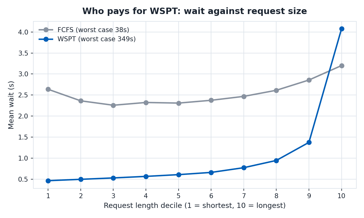
Figure 8. Where the tradeoff really lives. Plotting mean wait against request-length decile, FCFS is almost flat (2.64s for the shortest tenth, 3.20s for the longest) because it is indifferent to size by construction. WSPT is steeply graded: 0.46s for the shortest tenth rising to 4.08s for the longest. And the worst case is the headline: 38s under FCFS against 349s under WSPT, close to a tenfold difference.

So Dynamo's claim is right, and my figure 7 was measuring the wrong statistic. "FCFS optimises tail TTFT, no request waits longer than necessary" is a statement about the worst case and about fairness across sizes, not about p99 of a class. p99 is still dominated by ordinary queueing, which WSPT genuinely improves. The starvation WSPT causes is concentrated in the last decile and the maximum, which is exactly where the theory in section 5 says SRPT-family policies hurt. If your SLA is written on mean or p99 TTFT, use WSPT. If it is written on a hard per-request deadline, or you have customers whose requests are systematically long, FCFS within the class is protecting you from a complaint you have not had yet.

This is also the practical case for the two-level design rather than a single index rule. Put the long-request-heavy tenant in its own class with a guaranteed quantum, and you get WSPT's mean-latency win inside each class without WSPT's worst case crossing tenant boundaries. Isolation from DRR, efficiency from Smith's rule, and neither one asked to do the other's job.